


Author:
Publication:
Data collection requires follow-on signal processing, namely filtering. It is common to remove a specific component or frequency bandwidth of a data set in order to separate extraneous from pertinent data. Proper filtering is necessary to achieve meaningful and accurate data for follow-on analysis, especially for analytics such as power spectral density. This Product How-To article explains how to remove signal data artifacts using a finite impulse response notch filter and a Python-based math platform.
Specifically, it outlines a method of notch or bandstop filtering used to parse out very specific frequency components in a test data set with minimal impact to surrounding relevant data.
In this method, data was collected using a wireless battery-powered LORD Sensing Systems SG-Link-OEM LXRS electronics package connected to a torque strain gage rosette on a drive shaft. The drive shaft rotated at a high rate of speed, and the instrumentation package was configured to measure dynamic and static torque during periods of operation. A typical node operating within a LORD wireless network is synchronized via a broadcast timing source, and is assigned a specific “window” to sample and transmit its wireless data within (see Figure 1).

In this case, it was desirable to maximize sample rate, so the wireless node was configured to collect data continuously at 512 Hz. The resultant data exhibited an artifact that resulted from the data transmission window overlapping the sample window. In essence, the wireless system was radiating RF energy onto unprotected portions of the strain gage rosette wiring that then behaved like an antenna. This self-inflicted RF energy caused strain gage bridge excitation that was then measured by the wireless sensor. The subsequently induced data artifact appeared in all data sets since it is a function of sample rate. Spikes and consequent harmonics are visible in the normalized time series plot (see Figure 2) and corresponding frequency domain (see Figure 3).


Figure 3: Spikes and harmonics are also visible in the corresponding frequency domain for the data in Figure 2.
The data artifact is clearly not the result of a mechanical system vibration due to the lack of sidebands, any discernible bandwidth, and the fact that the wireless sensor was transmitting in 32 Hz intervals. Our data showed the highest energy levels at 32 Hz, followed by frequency content at every 32 Hz harmonic until filtered out by the hardware 200 Hz anti-aliasing filter. The data is usable as is, but a better method is to filter out positively identifiable anomalies using a specifically designed signal processing algorithm. (Note: Within this paper, the terms notch and bandstop are used interchangeably.
FIR Filter Design
The goal of this filter application was to clearly attenuate the amplitudes of the artifact frequency content, while minimally impacting the surrounding data. These parameters correlate to a window style filter of a significantly high order with limited off frequency ripple and a narrow transition region. A finite impulse response (FIR) function using a Kaiser Window was selected from Python for use in this filtering application.
The kaiserord function within SciPy requires two inputs: desired filter width normalized to the corresponding Nyquist value for the data set, and desired filter attenuation. This function then returns the variables needed to build a Kaiser Window: filter window width and beta parameter. The SciPy firwin function computes the coefficients for the FIR filter. Finally, the filtfilt function applies the windowed filter, using the previously generated coefficients, to the data set and outputs the filtered data. Notch filtering is achieved by building an array of frequency bandstop points normalized to Nyquist and passing them to the firwin function. (This code is shown in Figure 4 and was based off an example on SciPy.org Cookbook.)

Some adjustment is required for the filter width and attenuation depending on the data set and the desired effect. Higher artifact energy levels obviously require more attenuation with respect to nominal data magnitudes. Filter width is necessary to adjust depending on how much attenuation is achieved, and in an effort to minimize the effect to surrounding “real” data. It is also important to note that linear FIR filter functions typically exact a phase shift on the output data. Instead of trying to adjust data sets to align in the time domain, this problem is easily corrected by applying a linear filter twice: once in the forward direction, and once backwards. The net effect is zero phase shift with the filtered data.
Filter Results
Once coefficients were appropriately applied, the overall filtering function had exactly the desired effect. Data artifact energy levels were minimized at bandstop frequency windows. Most data set anomalies were removed with a 700-1000 order filter (see Figure 5).

Input time series data and frequency content are compared to filtered time series and frequency content in Figure 6, Figure 7, and Figure 8. It is readily apparent in the frequency domain plot where the filter attenuated the output data set. Amplitudes are normalized in all data sets. Resultant data alignment showed no phase shift, and clear removal of 32 Hz data RF artifacts.


Figure 8: Frequency Domain Unfiltered (a) vs. Bandstop Filtered (b) Data
Conclusions
Filtering via this method proved to work exceedingly well for this data set and this application where very specific bandstop frequencies were targeted for attenuation. Through the process of understanding the filter, designing it, and using it on a data set, several points were apparent.
For a data filter to work properly with a minimum impact to relevant data, it is important for the user to fully understand the filter function, coefficients, and effect each coefficient adjustment has on the data. Failure to understand may lead to an erroneous output, or the attenuation of relevant data. There are many online resources to reference in regard to filter design and pre-built functions available to use, especially for Python applications.
While the root cause of this exercise was induced by excess RF energy on an unprotected antenna, it is important to note that post processing was able to adequately filter the test data. A separate hardware solution was identified and implemented immediately after this problem was discovered.
Of consequence to the total algorithm, but not specific to the filter, is the effect prime number inputs have on a Discrete Fourier Transform (DFT) function computation time. While a DFT function on a non-prime input will execute with N*log(N) operations, a prime input will take N2 operations. This exponential increase in computation time can adversely affect the post processing effort; in this case it took 700,000 times as long. There are two obvious solutions to this problem: remove beginning or end data set values until a non-prime number of input points is achieved, or pad the input data set with zero values at the end until reaching a non-prime number of total points.
Notch filtering is a viable way to remove undesirable data artifacts or signal noise. For this application, it enabled the removal of a high energy data artifact that was an order of magnitude greater than the frequency content of interest. It also removed the obvious 32 Hz component from the time series data set, making the data more relevant and easier to correlate to actual shaft dynamics.
Notes:
1. Full Algorithm for data filtering can be found here
2. SensorCloud was used to deposit and maintain all data sets.
3. MathEngine was used to run analytics on cloud based data sets.
4. Python computer language was used for all coding.
About the Author
Dan O’Neil is a graduate of Norwich University, and has worked as an Air Force aircraft structural repair engineer, flight test engineer, and development engineer. He currently works for LORD Sensing Systems in Williston, VT as a Senior Mechanical Engineer developing wireless solutions for aeronautical and industrial customers. Dan lives in Vermont with his wife Megan.